Packages

First, we note that instead of library(), we will use import ____ to load in packages. Additionally, to use functions from these called modules, we will have to specify the module name in front of the function (e.g. math.sin() instead of sin()).

To install the packages, there is no install.packages() equivalent. Thus, we head to the Terminal section of RStudio and enter pip list to check what packages we already have. It seems that while I have pandas already installed, I want to install matplotlib and numpy for the future, so I run pip install matplotlib and pip install numpy.

import numpy as np
import pandas as pd
import matplotlib

Perfect, all the packages have imported properly, we can proceed forwards!

Initial Data Exploration

Now onto data processing. Since reading in a csv file gets complicated on this website, I will use an in-built dataset. After a quick search, we find documentation for the sklearn library, which discusses many datasets that are shared with R, including iris.

After running pip install statsmodels in the terminal, we can now do the following:

from sklearn.datasets import load_iris
iris_raw = load_iris()

# Load iris into a dataframe and set the field names
iris = pd.DataFrame(iris_raw['data'], columns=iris_raw['feature_names'])

Here, we used the pandas library to convert the data into a data frame, then printed the first few rows. While I’m not entirely clear how the DataFrame function works, I’m certain we’ll get to that shortly.

Now that we have a dataset, we return to the workshop materials.

With a dataset on hand, we explore the basic functions that we’re familiar with for R.

• head() = .head()
• tail() = .tail()
• summary() = .describe()
• names() = .columns
• dim() = .shape

iris.head(3)

##    sepal length (cm)  sepal width (cm)  petal length (cm)  petal width (cm)
## 0                5.1               3.5                1.4               0.2
## 1                4.9               3.0                1.4               0.2
## 2                4.7               3.2                1.3               0.2

Alright, perfect. The functions do have arguments like in R (e.g. iris.head(3) to get 3 rows only), but again, we can learn those as we go.

Data Manipulation

Next, we want to learn about all the data wrangling abilities we had with the dplyr function in R. From the workshop notes, we’ll continue to use pandas for now.

First, we observe that instead of using $ to specify variables, we have to index with []. Instead of using a vector (c('var1', 'var2')) to store multiple column names and call them together, here we will have to use a list (['var1', 'var2']).

Creation of a new variable seems to be the same as in base R. For example, instead of df$new = df$var1 + df$var2, we will do df['new'] = df['var1'] / df['var2']. Seems straightforward enough!

Several functions are also listed:

• filter() = .query()
• sort() = .sort_values()
• rename() = .rename()
• summarize() = .agg()
• group_by() = .groupby()
• is.null() = isnull()

Let’s give the filter and summarize functions a try!

iris_red = iris.query("sepal length (cm) > 5.0")

We’ve run into our first error! Turns out query requires no empty spaces in variable names, so after a quick fix, we can proceed onwards.

# Change the column names to remove spaces
iris.columns = ["sepal_length", "sepal_width", "petal_length", "petal_width"] 

# Filter for sepal lengths at least 5 cm long
iris_red = iris.query("sepal_length > 5.0")
iris_red.head(3)

##     sepal_length  sepal_width  petal_length  petal_width
## 0            5.1          3.5           1.4          0.2
## 5            5.4          3.9           1.7          0.4
## 10           5.4          3.7           1.5          0.2

Seems like the filter function is working as intended. We do note that the query argument is a bit less intuitive than for filter(), but nevertheless, it is manageable.

Next, we want to try the summarize() equivalent.

# Calculate mean of sepal length and median of sepal width
iris.agg({"sepal_length" : np.mean, "sepal_width" : np.median})

## sepal_length    5.843333
## sepal_width     3.000000
## dtype: float64

# Calculate min and max values of all the variables
iris.agg(['min', 'max'])

##      sepal_length  sepal_width  petal_length  petal_width
## min           4.3          2.0           1.0          0.1
## max           7.9          4.4           6.9          2.5

This will require some getting used to. The documentation for .agg discusses other arguments and options, but this gives us an idea of what we’re dealing with.

Now, we know the select(), mutate(), summarize(), and group_by() equivalents. I consider these the fundamental functions, so things are looking good!

Visualization

Onto section 4 of the workshop!

This workshop uses the seaborn library, so we will use that for now since it supposedly closer to ggplot2. We will explore matplotlib at another time.

Our goal will be to explore the basic plots, axis/title labeling, faceting, and coloring.

import seaborn as sns

# We need to import this to show the plot
import matplotlib.pyplot as plt

# Create Petal Length vs Sepal Length scatterplot with regression line
sns.lmplot(x="sepal_length", y = "petal_length", data = iris)

plt.xlabel('Sepal Length')
plt.ylabel('Petal Length')

# Display the plot (required for R Markdown to show)
plt.show()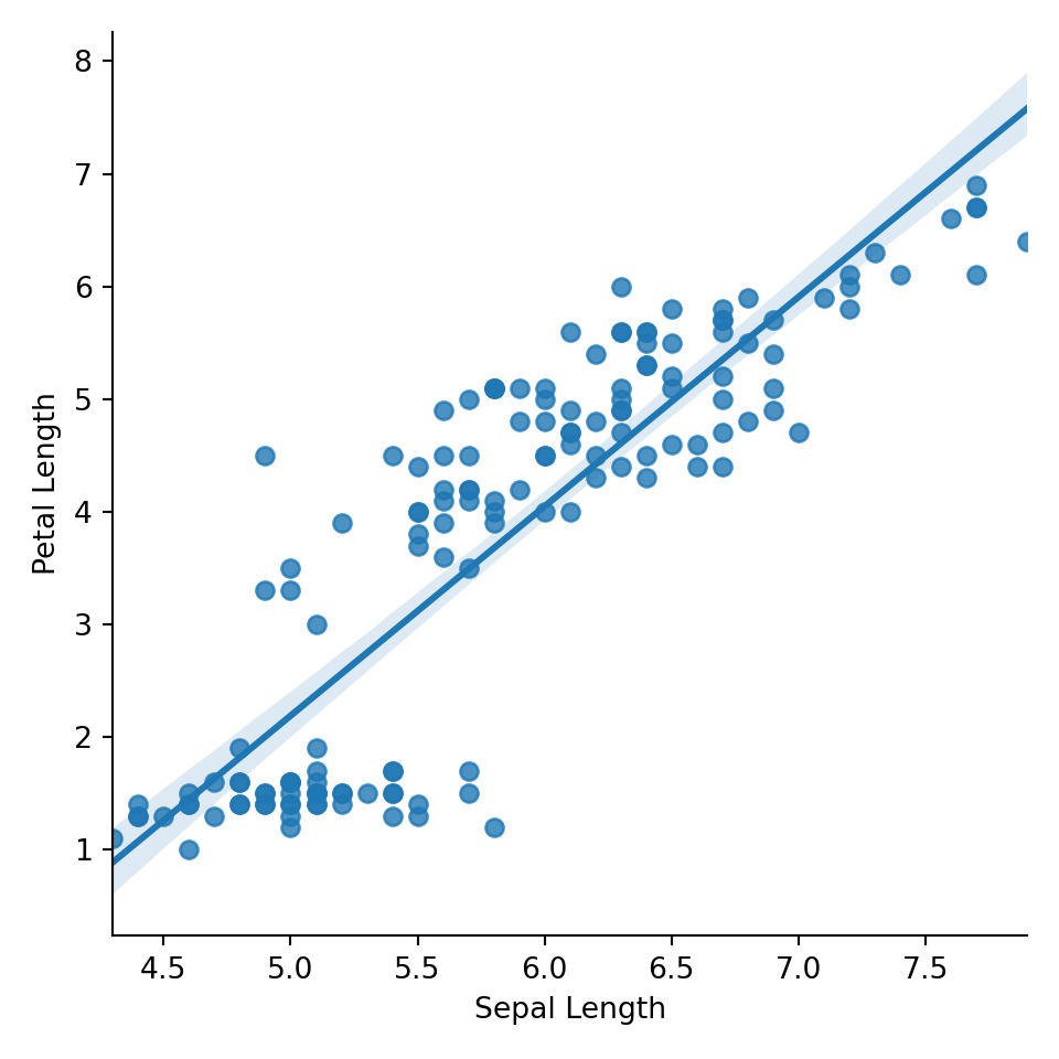

The code seems to be more akin to base graphics in R. Regardless, it seems to be working appropriately. Next, we review how to facet these graphs.

The iris dataset here doesn’t actually have a species name variable, so we create a categorical variable to fill that need.

After exploring different options to create the new variable efficiently, we explore the .insert() function. Since iris has 150 rows, we create a categorical variable with 2 unique values (75 rows each).

# Create the species variable which switches between Setosa and Virginica
iris["species"] = ['Setosa', 'Virginica']*75
iris.head(3)

##    sepal_length  sepal_width  petal_length  petal_width    species
## 0           5.1          3.5           1.4          0.2     Setosa
## 1           4.9          3.0           1.4          0.2  Virginica
## 2           4.7          3.2           1.3          0.2     Setosa

It is successful! So, we now create the faceted graph.

# Create Petal Length vs Sepal Length faceted graph with regression line
sns.lmplot(x="sepal_length", y = "petal_length", 
           col = "species", hue = 'species', data = iris)

plt.xlabel('Sepal Length')
plt.ylabel('Petal Length')

# Display the plot (required for R Markdown to show)
plt.show()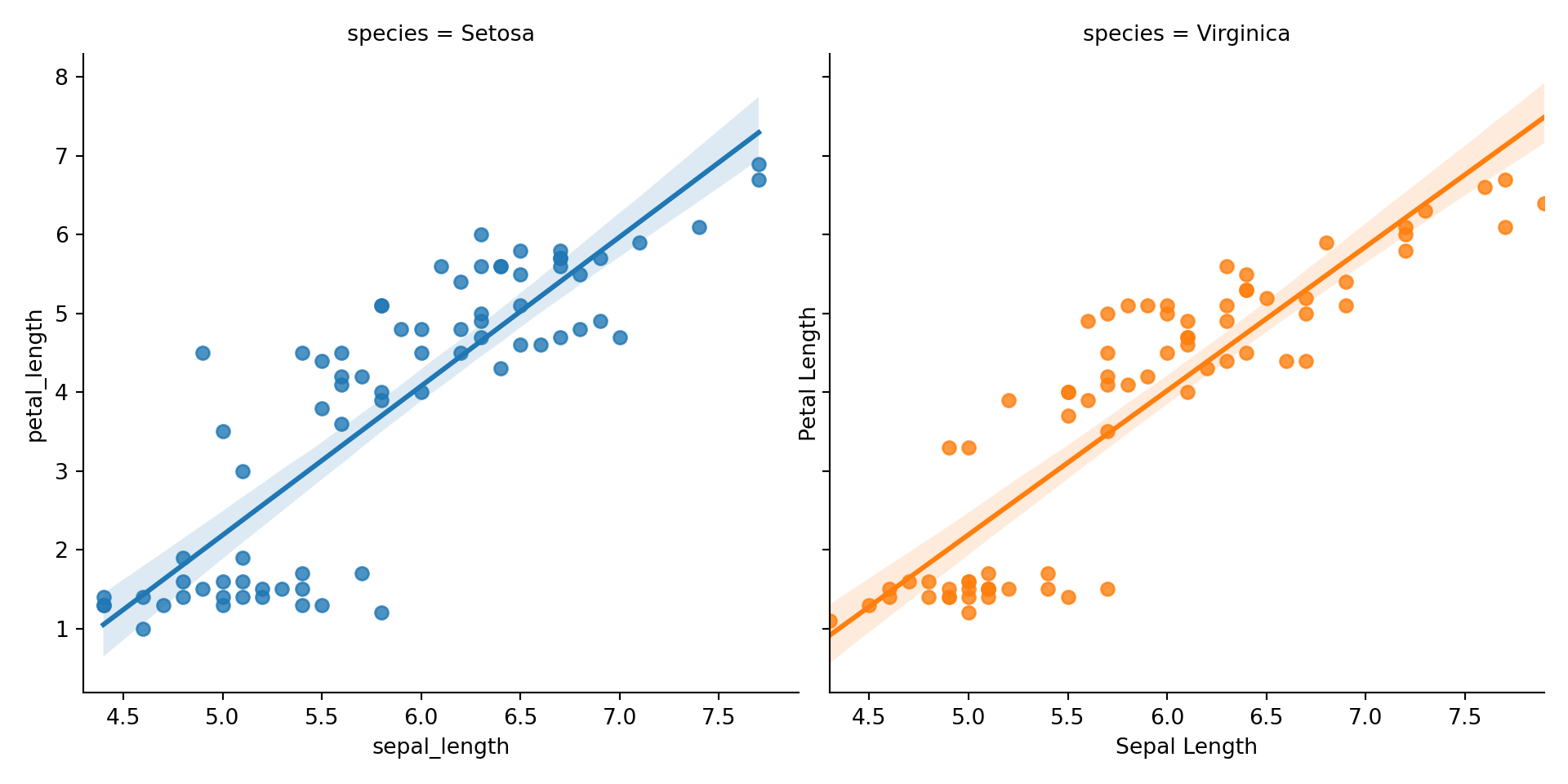

It works! While I have no doubt that eventually there will a struggle to figure out details like font size, text labeling, this seems like a great point to stop when there isn’t a definitive end goal in mind. We will continue to explore plotting in our next post on this subject.